
A few years ago, in2Dredging developed the Pumps ‘n Pipeline (PnP) estimating tool, which can be used to accurately estimate suction and discharge production. In this post, PnP’s results are introduced chronologically, so as to help describe how suction production rates can be estimated more accurately.
PnP has already been explained at a high-level in the classic post ‘How Pumps and Pipeline Estimating Tool Works’.
Pump Behaviour
For any PnP calculation, the pump behaviour is described by providing both pump head and pump efficiency regression coefficients. To estimate suction production more accurately, the Nett Positive Suction Head required (NPSHr) curve must also be provided. This curve provides information on the pump’s suction characteristics at different flow rates.

Suction Performance
Polynomials established through regression analysis, enable the calculation of the NPSHr curve for both the minimal and nominal pump revolutions. Once the NPSHr curves have been calculated, they can in turn be used to calculate the limiting vacuum curves.
Limiting vacuum is the pressure at which the pump just starts to cavitate and lose performance. It represents a physical bottleneck for production rates. Severe cavitation can have serious negative impacts on the pump’s performance and its lifespan.

The limiting vacuum can be determined from the Suction Performance graph for both minimum (i.e. 500 rpm) and nominal pump revolutions (i.e. 540 rpm). The limiting vacuum can also be determined for both water and mixture density, which in this example is assumed to be 1,400 kg/m3. Note that Limiting vacuum is density dependent.
In addition, from the above graph one can also already ascertain that the limiting vacuum increases by approximately 10 kPa at a flow rate of 0.6 m3/sec when the pump revolutions are reduced to a minimum.
Production Limitations
Figure 3 below shows Production Limitations by graphing flow rate on the horizontal axis and the production rate on the vertical axis. The colours on the graph represent the working areas. The green working area is considered “possible”, the orange is considered “challenging” and red is considered “impossible”.
Figure 3 also presents three parabolas, which represent the limiting pump vacua ranges from 40 to 60 kPa. These ranges were derived from Figure 2 above.
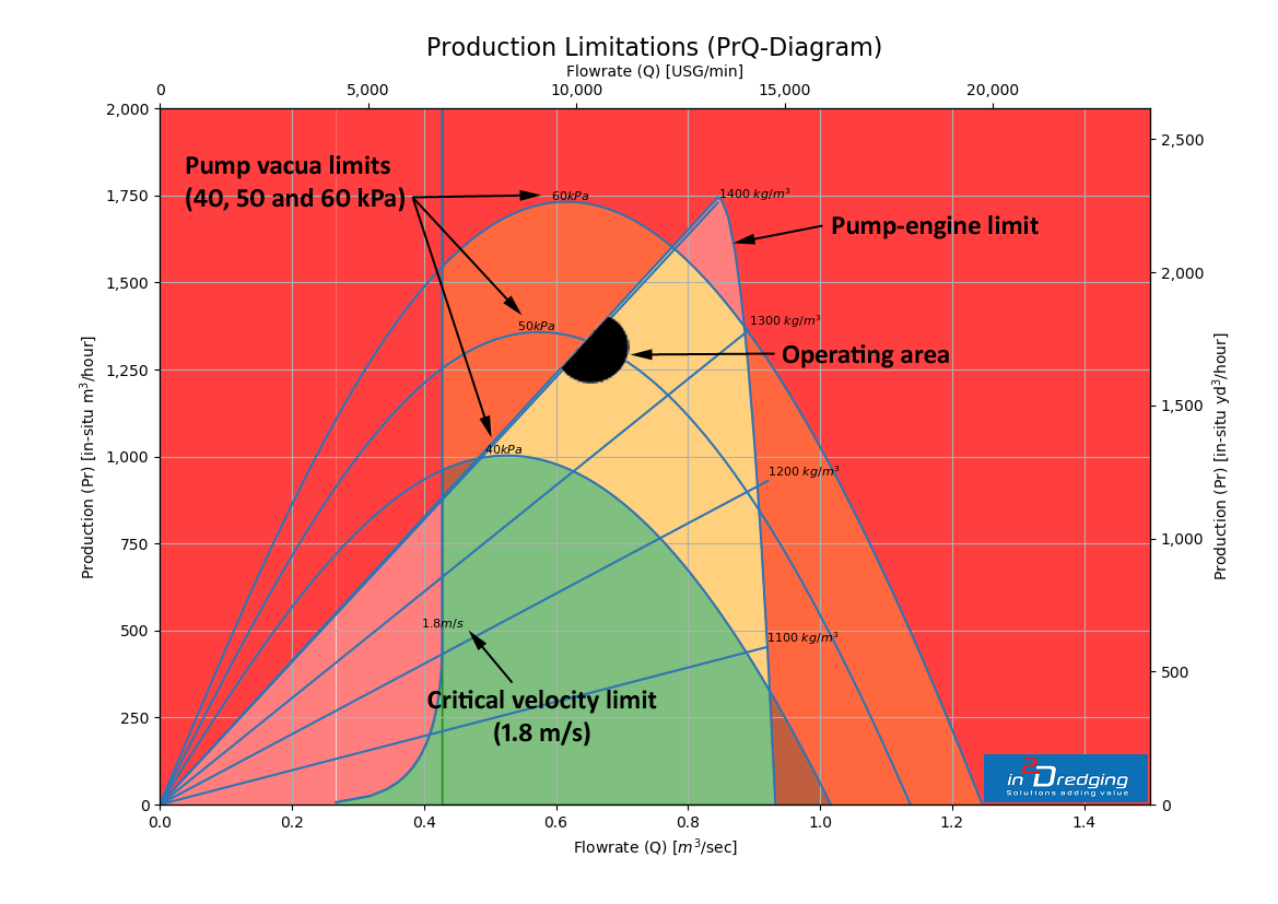
With the Production Limitation graph depicted in Figure 3 above, one can deduce at a glance the achievable production rates (i.e. ~1,250 m3/hour) in “challenging” conditions. The graph also shows that mixture densities just below 1,400 kg/m3 and flow rates just above 0.6 m3/sec result in maximum achievable production rates, as per the vacuum production parabolas.
In the example depicted in the above graph, one can see that production is limited by the mixture density forming limit, which is assumed to be 1,400 kg/m3, and the pump’s vacuum (<53 kPa @ 0.6 m3/sec). Therefore, reducing the pump revolutions would increase the production rate, not only by increasing the limiting vacuum but also by lowering the mixture flow. This in turn makes more vacuum available to lift a higher mixture density, thus providing higher suction production rates.
Read more on how Pumps ‘n Pipeline (PnP) can support you to not only accurately estimate suction and discharge production, but also with bottleneck assessments and optimising production rates.